The archetypal beginner example used to explain the GPU architecture shows how loop iterations can be executed in parallel by multiple threads. For instance, consider this snippet, taken and slightly adapted from [2]:
1 | for i in 1..N: |
Intuitively, each iteration is independent of the others. This is why it is possible to run them across different threads. In CUDA, the loop is replaced with a “kernel”, i.e. a function that runs in a single thread, as illustrated in this piece of code:
1 | void my_kernel(int *a){ |
In a couple of posts inspired by [4] (here and here), I informally described how category theory can be used to expose parallelism in computer programs. So, I was curious to know if we can use the same gadgetry introduced there to parallelize the code above, automatically. In the rest of this post I want to study this problem and sketch a solution. You don’t need any knowledge of the GPU architecture to follow my ramblings. However, if you are interested, you can find an introduction in [1].
There is another work where Category Theory is applied to GPU computing. In [3], the authors present a data structure for hypergraphs that can be efficiently implemented on parallel hardware such as GPUs. If I understand correctly, what they do is different from our present goal. To put it simply, they use GPU-optimized hypergraphs that runs efficiently on GPUs. However, our goal is different: we want to build a compiler that also uses hypergraphs as an intermediate representation, but the final product is GPU-optimized code, not necessarily the compiler itself.
Representing arrays in data diagrams
First of all, we need to represent arrays in string diagrams. We follow [4] where programs are modelled as a data structure consisting of two layers, circuits and tapes, that represent data and control in programs, respectively. For simplicity’s sake, we consider only structured programming languages where control flows are restricted to a particular subclass, see our previous post for details.
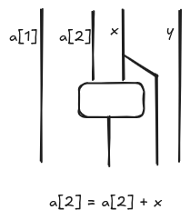
A data diagram is a string diagrams where wires are data and boxes operations on data. More specifically, wires represent tuple of types. Hence, it is natural to look at arrays as bundles of wires of the same type as illustrated below for the command a[2] = a[2] + 1.
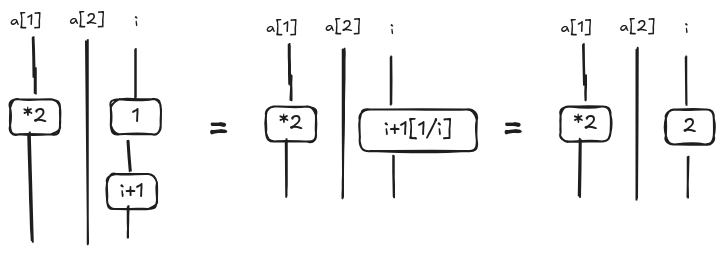
The main challenge is to describe how array elements can be accessed dynamically, that is, when the index is not a number but another variable, e.g. a[i]. Let’s suppose that a is an array of elements of type T and i is an index, then we define the expression a[i] (i.e. read an array element) as follows:
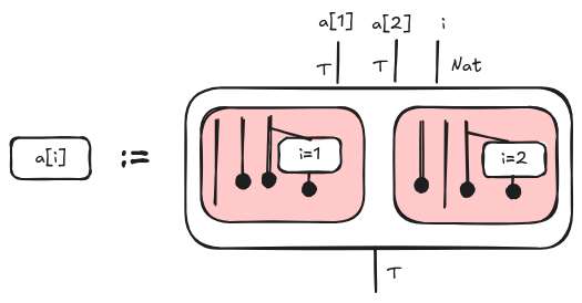
Intuitively, each red box represents alternative control flows dependent on the value of i. At most one condition i=n in each box can be evaluated to True for a given value of i; so at most one red box is different from the empty relation. If the index is out of bound, the diagram is the empty diagram.
We can write it also as a formula $a_i = \sum_{n \in N} c(i=n); \mathit{proj}_n$ where $c$ is the condition diagram and $\mathit{proj}_n$ discards all the wires but the $n$-th one.
Now we have to define a diagram for assignments a[i] = e. We use the same trick: the element of the array that is written is condionally picked up using alternative control flows in such a way that at most red box is non empty for a given value of i.
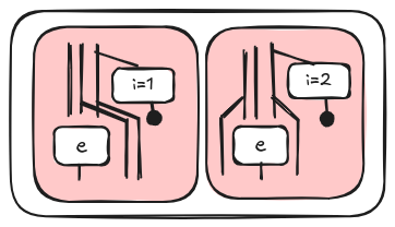
The formula is a bit more complex in this case, but it should be pretty intuitive. Note that we simplified it a bit assuming that we have only one array always on the left. In this blog post we don’t consider the general case.
$$
\sum_{n \in N} c(i=n); \blacktriangleleft_{1 \ldots n-1} \otimes \mathit{id}
\otimes \blacktriangleleft_{n+1 \ldots N};id_{1 \ldots n-1} \otimes \mathcal{E}(\Gamma \vdash e) \otimes \mathit{id}_{n+1 \ldots N}
$$
Generating parallel code
First, we rewrite the program above with a syntax closer to the one in [4]: a for is just syntatic sugar for a while, as it is well known.
1 | i = 1 |
The diagram is the following one. The blue box is a Kleene operator (see [4], basically it is a transitive closure).
In order to simplify the diagram, we unfold the Kleene/While operator. As it is common in the literature, while c do d can be defined recursively as if c then (d; while c do d) else skip. This is the basic idea behind unfolding. In the following picture, we show a single-step unfold corresponding to the first iteration of the loop.
Now, we can simplify the diagrams applying some rewrite rules. Let’s consider the first part of the unfolded diagram $\mathcal{E}(\Gamma \vdash i\mathit{:=}1;c(i<N))$. Graphically, it is represented in the picture (1) below.
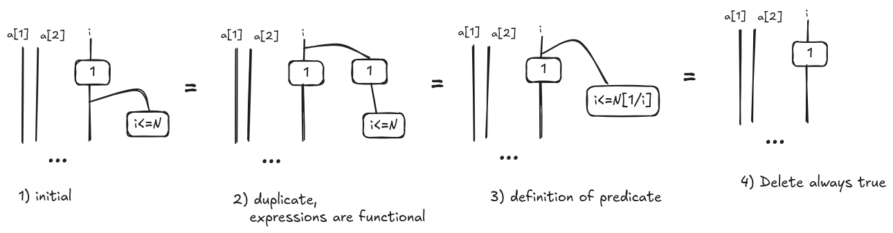
Since an expression is a function and not a predicate, we apply the duplicate rule (2). Because $\mathcal{E}(\Gamma \vdash e);\mathcal{E}(x \vdash P(x)) = \mathcal{E}(\Gamma \vdash P(x)[e/x])$ for Lemma 11.4 in [4], we can simplify the diagram as in (3) and obtain $\mathcal{E}(\Gamma \vdash i\leq N[1/i]) = \mathcal{E}(\Gamma \vdash \mathit{True})$; so, the right branch is always true and it can be pruned. We want to observe that these rewrite rules resemble constant propagation, a well-known optimization technique in compilers. This is not a coincidence, we will show in subsequent posts how other compiler optimizations can be described in terms of rewrites on hypegraphs.
In a similar way, we can propagate expressions into convolutions because of their properties and the fact that expressions are functional. Then for each red box we can apply the simplification above.
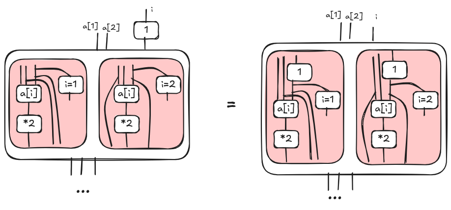
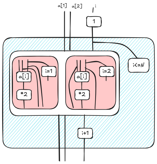
Now, we can simplify the conditions i=n in each red box as we did previously. However, at this time, at most one red box is a non empty relation. So we end up with a sum where at most one term is non zero. Hence, we can simplify the diagram removing the convolution as illustrated below.
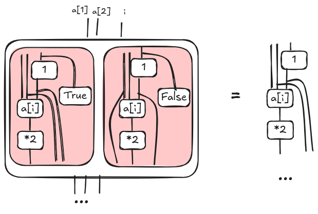
Now, we can expand a[i] applying the definition given in the previous section. The expansion reveals another convolution; we can remove the new convolution as we have just done above; drawing the steps is left as an exercise. Finally, we want simplify the node that increments i. This is similar to the simplification for predicates, but this time we use the analogous Lemma 11.3 in [4].
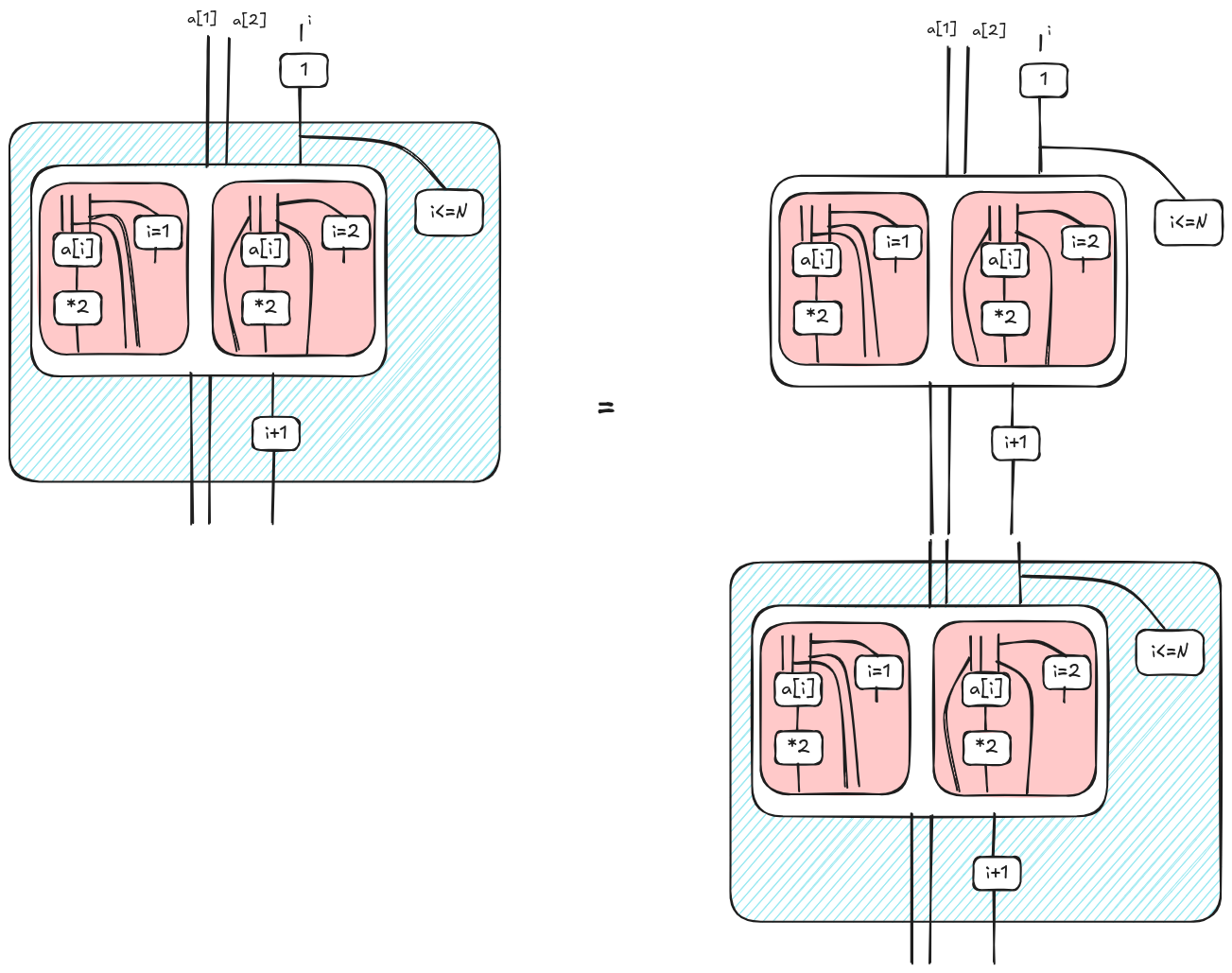
We repeat the same steps for the other iterations until we don’t have anything else to unfold, i.e. at some point $i<=N$ will be false making the “continuation” empty. Here, we summarize the steps.
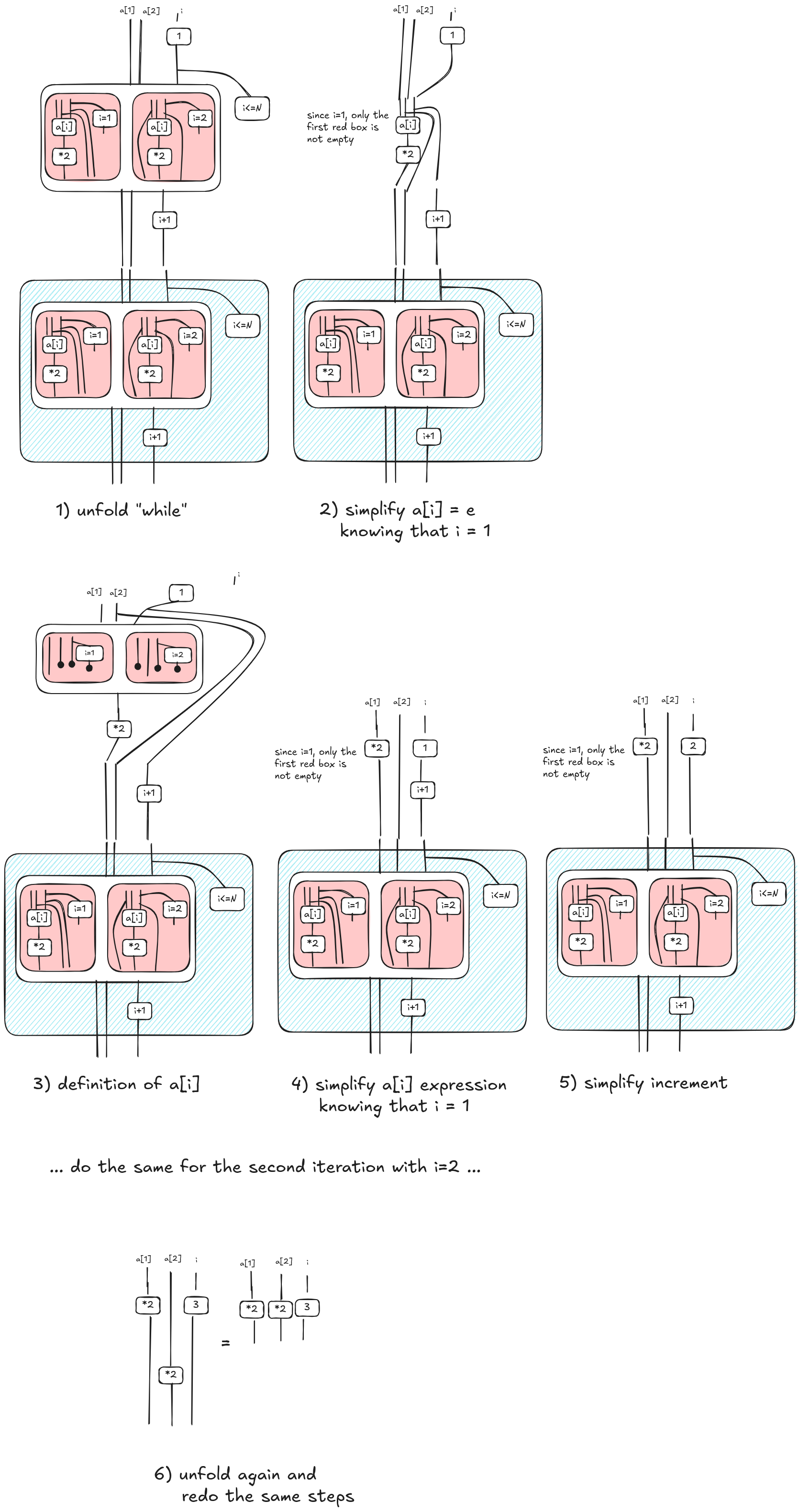
Eventually, we get a diagram where we apply “in parallel” *2 to each element of the array. This is what we wanted to obtain. The procedure generates an artifact 3 corresponding to the last value of i; since this artifact is not used elsewhere, it can be trashed.
Final notes and a disclaimer
Despite the example is pretty simple, I think it is cool. For example, if iterations are data dependent, the parallelization wouldn’t be possible and the graphical language would catch it. What I find also fun is that GPU threads are actually wires in our graphical formalism: so we have preserved also the metaphors!
The examples provided here primarily cover a happy path, and a more formal treatment would require significantly more attention to detail and edge cases. The posts I write here are essentially an attempt at “learning in public.” Think of them as sharing unreviewed notes, the kind that would typically reside privately in a paper notebook. My reasons for doing so are twofold: to gather feedback and to connect with like-minded individuals. I am not yet certain about their correctness and would greatly appreciate any feedback you might have.
References
[1] ENCCS, GPU Programming, accessed May 2025 online
[2] Paul Richmond, Introduction to GPU Programming, ICCS 2023 YouTube
[3] Wilson, Paul, and Fabio Zanasi. “Data-parallel algorithms for string diagrams.” arXiv preprint arXiv:2305.01041 (2023). pdf
[4] Bonchi, Filippo, Alessandro Di Giorgio, and Elena Di Lavore. “A Diagrammatic Algebra for Program Logics.” arXiv preprint arXiv:2410.03561 (2024). pdf