In this post, I want to share some initial ideas on surfacing parallelism in code, drawing inspiration from the category theory framework introduced in [3] and [4]. My approach will be informal, prioritizing intuition over strict mathematical details to make these concepts more accessible to a broader audience, particularly software engineers. In fact, the potential benefits of this theory extend to practical areas like compiler design (e.g. [5] shows related ideas). While aiming for clarity, there might be simplifications or unintentional mistakes. Think of this as an idea-sharing session, and I’d love to hear your thoughts and reactions!
Let’s look more closely at what I mean with the expression “surfacing parallelism” using a simple example. Consider the code snippet below,
1 | x = 10000 |
It consists of two if-then-else blocks that may perform expensive operations. The second if-then-else is executed only after the computation of the former if-then-else has terminated. However, since the two if-then-else blocks are independent from each other (i.e., they work on different variables), we could run them in parallel. The problem we want to discuss here is how a sequential program can be rewritten into a semantically equivalent program where independent code blocks are carried out in parallel. We want to do that in order to speed up the overall computation. Indeed, we expect that two parallel heavy computations will run faster than when they are executed in sequence.
Our working example is adapted and simplified from [1] where the author observed that surfacing parallelism can be done in a systematic way by applying precise rewrite rules to computer programs. This is possible thanks to an interesting algebraic duality between data and control (more later) that was discovered many decades ago in [2]. In the rest of this post, we will repropose a similar exercise in the more modern setting of tape diagrams [3] that simplifies our task a bit.
Tape Diagram Semantics
A context $\Gamma$ represents a binding between variable names and types. In our example, $\Gamma=x \in \mathit{Nat}, y \in \mathit{Nat}$. Sometimes, we are interested only in types; then we define a function $\epsilon$ that takes a context and returns only the type side of a context. For our choice of $\Gamma$ the type side is $\mathit{Nat} \times \mathit{Nat}$. If you are familiar with programming language theory, this is the gist of alpha conversion: variable names don’t change the semantics of a program so they are irrelevant for a computer (but they are not for humans!).
Intuitively, commands define functions from $\epsilon(\Gamma)$ to $\epsilon(\Gamma)$. For example, x = x - 1 corresponds to a function $\epsilon(\Gamma \vdash \mathit{x = x - 1})$ that takes values in $\mathit{Nat} \times \mathit{Nat}$ to values in $\mathit{Nat} \times \mathit{Nat}$. More precisely, $(n, m)$ is sent to $(n-1, m)$ for each $n$ and $m$ in $\mathit{Nat}$.
We can represent functions of this type graphically using string diagrams. For x = x - 1 we get the following diagram where, wires are types and boxes are functions or relations. Just for notational convenience, we label wires with their corresponding variables.
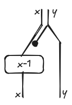
I think it is pretty intuitive. We need to read x and not y (that is why y is discarded) in order to evaluate the right hand side of the assignment. The result of the assignment overrides the original value of x and produce a new value. The value for y is copied over and sent to the inner context because we may need it for evaluating other expressions downstream.
We can do the same for conditions like x > 0. In this case, x is not overwritten by x>0, but it is propagated to the inner context without any change. The predicate x > 0 is not a function, but a relation. If you want to understand how it works, please refer to [4]. The intuition here is that the diagram acts as a sort of filter, that is, it is defined for every value of x and y such that x > 0, otherwise it is the empty relation.

These diagrams tell us how we operate on data and from now on we will call them data diagrams. In a computer program, we don’t have only data but also control flow. For example, we need to represent alternative flows of data when we execute an if statement. Intuitively, control is another “layer” that wraps data. In [3], the authors introduced the graphical language of tape diagrams where data diagrams are wrapped by a red tape. We call tape diagrams just control diagrams here to emphasize the application to the semantics of programming languages. The first if-then-else is represented as follows.
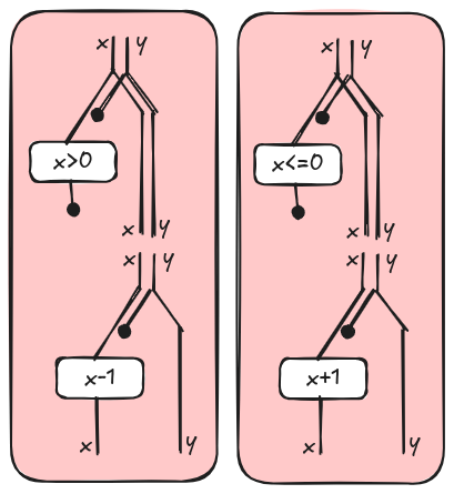
The two juxtaposed control diagrams capture the idea of “alternative” computations. We run either the then branch or the else branch, but not both of them! This is different from two juxtaposed data diagrams that, instead represent, data independency, e.g. things that can happen at the same time. This is the duality between data and control we were referring to at the beginning.
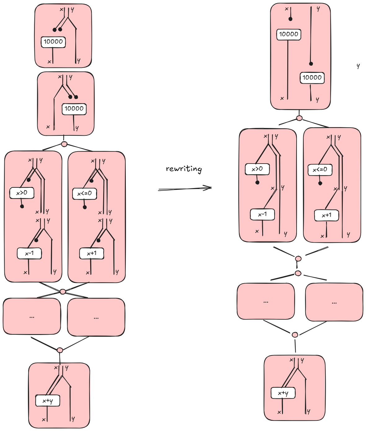
Now, if we put everything together, the control and data digram for our example is the diagram on the left in the picture below. Note that we introduced some special nodes for branching out and merging computations and we omitted the diagrams for the second if-then-else that are left as an exercise.
Tape diagrams are a special kind of algebra and can be manipulated applying some laws in the same way we used to do in highschool with polynomial equations. From a computational point of view, an algebra is nothing else than a data structure with some operations. For example, a rule says that, if we duplicate some data and then we discard one result, it is the same as doing nothing on the data. We can apply this rule to simplify our diagram a bit. For example, an assignment where some variables are not used can be simplified applying a rewrite rule as indicated below.
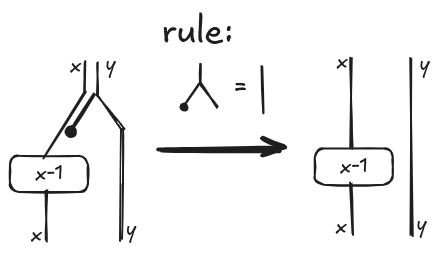
The result of applying this rule to our main example is shown in the above diagram on the right.
Well, surfacing parallelism is something similar. We apply some rewrites to the diagrammatic representation of a computer program that preserve the semantics. In the next section, I’ll give the basic intuition.
Surfacing parallelism
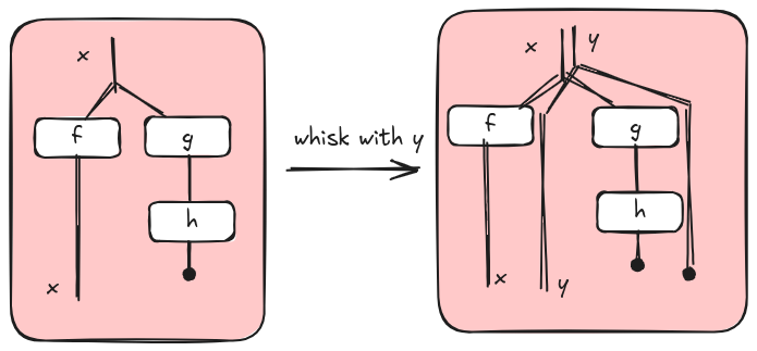
In [3], the authors introduce the concept of whiskering. I think the original motivation for whiskering was to explain how the two monoidal structures of tape diagrams distribute over each other. However, if these words sound too obscure, it is more intuitive to think about whiskering as a sort of operator on diagrams that increases parallelism by interleaving computations. For example, suppose that we have the tape diagram on the left with context x, we can extend its context with y whiskering the diagram on the right (or on the left) obtaining the diagram on the right with context xy. The new whisked diagram is “equivalent” to the original one because we don’t change what we do on x and we don’t do anything on y. So why is whiskering useful if nothing changed? It is useful because, after whiskering, we have an extended context xy and we can interleave computations over x with computations over y.
Let’s consider a simple example of two parallel computations as in the following diagram (left). We use a green tape to highlight the fact that the left and the right are not alternative options, but they run in parallel.
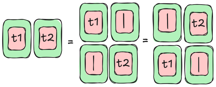
What does “running in parallel” mean? Intuitively, two computations are parallelizable if the order of execution does not change the behavior. In other terms, left and right are parallel if we can run left and then right (center diagram) or right and then left (right diagram) without changing the result of the computation.
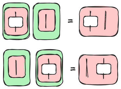
Basically, we run the left and we do nothing on the right or vice versa; in other terms, we are whiskering. The patterns “do nothing on the left” and “do nothing on the right” are quite important and deserve their own notation: $L_U(t)$ and $R_U(t)$ where $t$ is a generic tape diagram.
It is not too hard to convince ourselves than $L_U(t)$ (or $R_U(t)$) is the same as a data diagram when $t$ ends are not branching. Graphically, we have,
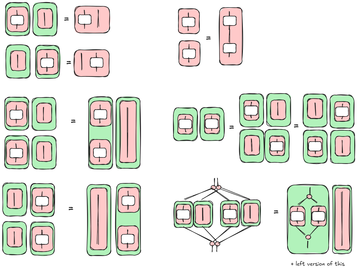
Here, we list some of the rules for tape diagrams that we can apply to surface parallelism. Please note that those rules can be derived by smaller ones defined in [3] and [4]. Here, we want to show the rewrite patterns that we need to apply in order to parallelize our example. So the rules are not the smallest building blocks, nor the set is complete.
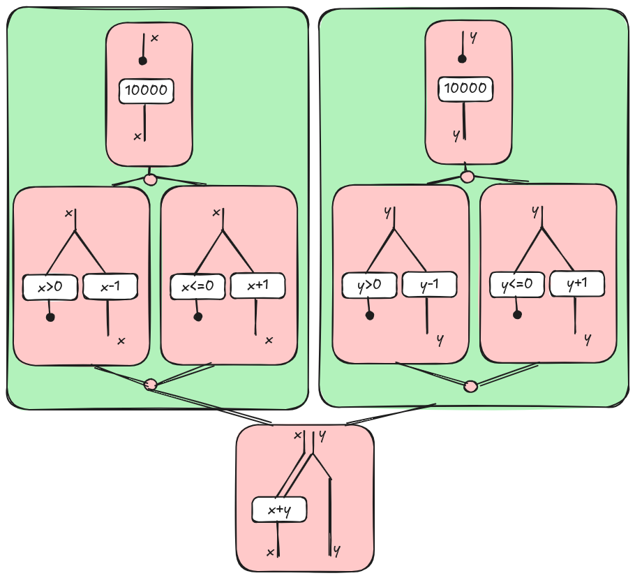
The final result is the following diagrams where we have two “parallel” if-then-else blocks as wanted.
Post Scriptum
In this post, I have tried to convey the intuition about these ideas. I must admit that I used a little poetic license to tell this story. I hope I will find some more time in the future for a more formal post, but I cannot promise anything.
In [4] and [5], the green tapes do not exist in the graphical language of diagrams. There exists an operation $\otimes$ on tape terms that is what we wanted to represent as a green tape. In some sense, we can consider green tapes as syntactic sugar, but it might be convenient to represent them graphically because of their interpretation as “parallel” computation. I can anticipate that the green tape is useful to model unstructured programming languages (those with gotos); for structured programming languages it is not strictly required: I am going to talk about this stuff in another post.
Finally, for the brave ones, I’ll copy here the algebraic expressions corresponding to the pictures. I don’t indend to explain their meaning, please read [4] and [5] if interested. I report them here just for my future myself. ;)
Starting expression
$\epsilon(\mathit{xy} \vdash \mathit{x=1});\epsilon(\mathit{xy} \vdash \mathit{y=1});$
$(c(\mathit{xy} \vdash \mathit{x>0});\epsilon(\mathit{xy} \vdash \mathit{x=x-1})+c(\mathit{xy} \vdash \mathit{x<=0});\epsilon(\mathit{xy} \vdash \mathit{x=x+1}));$
$(c(\mathit{xy} \vdash \mathit{y>0});\epsilon(\mathit{xy} \vdash \mathit{y=y-1})+c(\mathit{xy} \vdash \mathit{y<=0});\epsilon(\mathit{xy} \vdash \mathit{y=y+1}));$
$\epsilon(\mathit{xy} \vdash \mathit{x=x+y})$
Simplify assignment (discard) and apply whiskering
$R_y \epsilon(\mathit{x} \vdash \mathit{x=1}); L_x \epsilon(\mathit{y} \vdash \mathit{y=1});$
$(R_y c(\mathit{x} \vdash \mathit{x>0}); R_y \epsilon(\mathit{x} \vdash \mathit{x=x-1})+R_y c(\mathit{x} \vdash \mathit{x<=0});R_y \epsilon(\mathit{x} \vdash \mathit{x=x+1}));$
$(L_x c(\mathit{y} \vdash \mathit{y>0}); L_x \epsilon(\mathit{y} \vdash \mathit{y=y-1})+L_x c(\mathit{x} \vdash \mathit{y<=0});L_x \epsilon(\mathit{y} \vdash \mathit{y=y+1}));$
$\epsilon(\mathit{xy} \vdash \mathit{x=x+y})$
Whiskering compose and Whiskering convolution
$R_y \epsilon(\mathit{x} \vdash \mathit{x=1}); L_x \epsilon(\mathit{y} \vdash \mathit{y=1});$
$R_y (c(\mathit{x} \vdash \mathit{x>0}); \epsilon(\mathit{x} \vdash \mathit{x=x-1})+c(\mathit{x} \vdash \mathit{x<=0}); \epsilon(\mathit{x} \vdash \mathit{x=x+1}));$
$L_x (c(\mathit{y} \vdash \mathit{y>0}); \epsilon(\mathit{y} \vdash \mathit{y=y-1})+c(\mathit{x} \vdash \mathit{y<=0}); \epsilon(\mathit{y} \vdash \mathit{y=y+1}));$
$\epsilon(\mathit{xy} \vdash \mathit{x=x+y})$
Reordering (W7 in [4])
$R_y \epsilon(\mathit{x} \vdash \mathit{x=1});$
$R_y (c(\mathit{x} \vdash \mathit{x>0}); \epsilon(\mathit{x} \vdash \mathit{x=x-1})+c(\mathit{x} \vdash \mathit{x<=0}); \epsilon(\mathit{x} \vdash \mathit{x=x+1}));$
$L_x \epsilon(\mathit{y} \vdash \mathit{y=1});$
$L_x (c(\mathit{y} \vdash \mathit{y>0}); \epsilon(\mathit{y} \vdash \mathit{y=y-1})+c(\mathit{x} \vdash \mathit{y<=0}); \epsilon(\mathit{y} \vdash \mathit{y=y+1}));$
$\epsilon(\mathit{xy} \vdash \mathit{x=x+y})$
Whiskering compose
$R_y (\epsilon(\mathit{x} \vdash \mathit{x=1});(c(\mathit{x} \vdash \mathit{x>0}); \epsilon(\mathit{x} \vdash \mathit{x=x-1})+c(\mathit{x} \vdash \mathit{x<=0}); \epsilon(\mathit{x} \vdash \mathit{x=x+1})));$
$L_x (\epsilon(\mathit{y} \vdash \mathit{y=1});(c(\mathit{y} \vdash \mathit{y>0}); \epsilon(\mathit{y} \vdash \mathit{y=y-1})+c(\mathit{x} \vdash \mathit{y<=0}); \epsilon(\mathit{y} \vdash \mathit{y=y+1})));$
$\epsilon(\mathit{xy} \vdash \mathit{x=x+y})$
Definition $\otimes$
$(\epsilon(\mathit{y} \vdash \mathit{y=1});(c(\mathit{y} \vdash \mathit{y>0}); \epsilon(\mathit{y} \vdash \mathit{y=y-1})+c(\mathit{x} \vdash \mathit{y<=0}); \epsilon(\mathit{y} \vdash \mathit{y=y+1})$
$\otimes \epsilon(\mathit{x} \vdash \mathit{x=1});(c(\mathit{x} \vdash \mathit{x>0}); \epsilon(\mathit{x} \vdash \mathit{x=x-1})+c(\mathit{x} \vdash \mathit{x<=0}); \epsilon(\mathit{x} \vdash \mathit{x=x+1}));$
$\epsilon(\mathit{xy} \vdash \mathit{x=x+y})$
References
[1] Stefanescu, Gheorghe. Network algebra. Springer Science & Business Media, 2000.
[2] Bainbridge, Edwin S. “Feedback and generalized logic.” Information and Control 31.1 (1976): 75-96. pdf
[3] Bonchi, Filippo, Alessandro Di Giorgio, and Alessio Santamaria. “Deconstructing the calculus of relations with tape diagrams” Proceedings of the ACM on Programming Languages 7.POPL (2023): 1864-1894. pdf
[4] Bonchi, Filippo, Alessandro Di Giorgio, and Elena Di Lavore. “A Diagrammatic Algebra for Program Logics.” arXiv preprint arXiv:2410.03561 (2024). pdf
[5] Reissmann, Nico, et al. “RVSDG: An intermediate representation for optimizing compilers.” ACM Transactions on Embedded Computing Systems (TECS) 19.6 (2020): 1-28. pdf