Matrix calculus for Milner's Bigraphs

This post is still draft and made public “as is” without any revision and any claim about its correctness and completeness. You can track changes and amends in git log.

If you spot any mistake or you want to discuss anything, feel free to drop me a line at mstn@posteo.org.

This is the first of (maybe) a series of posts about Applied Category Theory [2]. It is more a personal exercise to “learn by doing” than something to be taken seriously. As a case study, I chose bigraphs: my tentative program is to apply some interesting concepts illustrated in [2] in this particular case.

Bigraphs [1] are a formalism invented by Robin Milner to model space and communicating agents. Milner is more famous for other breakthroughs in theoretical computer science, such as $\pi$-calculus and ML programming language. He was working on bigraphs at the end of his career, but we find similar ideas even in some of his early works. My source about bigraphs is [1]. You can find the same content in Milner’s original papers available online for free.

Circuit-like diagrams can be represented as matrices, see for example [2]. Here, we want to explore a matrix calculus that could be seen as a generalization of bigraphs.

While in [2] matrices are used to describe relations between inputs and outputs, here matrices are a sort of dependency graph.

Probably, the connection between bigraph and matrix calculus is already known, even if I have not found anything on the Web. Anyway, it is interesting enough to write a blog post about it.

In [2] (I have not read it, I have only read the short summary on Wikipedia) a generalization of bigraphs is proposed where spatial relations are modeled with a relation instead of a function as in Milner. A matrix can represent a sort of relation between rows and columns. Hence, it could be similar to what I am describing here.

In this post I will introduce bigraphs and their interpretation as matrices in a quite informal way. Hopefully, if I find time, I will focus on Category Theory in next posts.

Informal introduction

The following picture taken from [1] (p.13) is an example of bigraph.

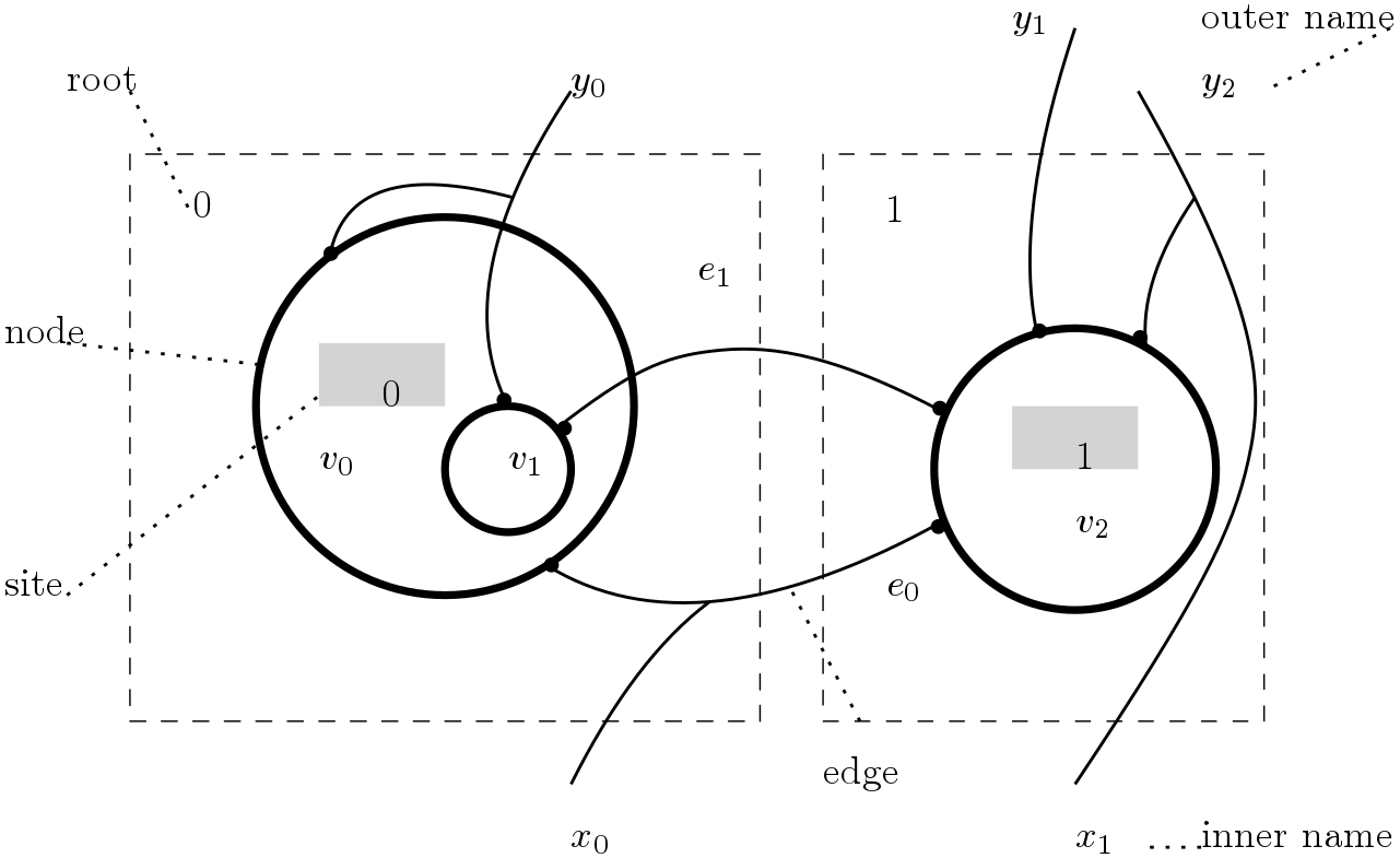
The component of a bigraphs are:

• Vertices $v_0, v_1, v_2, \ldots$. Vertices are interpreted as ambients and form a hierarchy (i.e. “within” relation).
• Vertices have ports (black dots) and ports are connected through edges $e_0, e_1, \ldots$. Edges are communication channels. Edges can cross boundaries.
• Roots $0, 1, \ldots$ and sites $0, 1, \ldots$ are outer and inner ambients, respectively. A site is a hole that can be filled with the root of another bigraph.
• Outer names $y_0, y_1, y_2, \ldots$ and inner names $x_0, x_1, \ldots$ are interfaces to connect ports to an external context and edges to internal ports.

The main insight behind bigraphs is that space and communication are independent. For example, I need to be in a particular room to get wifi access, but, when I send an email, the communication is independent (at the application level) from the spatial configuration of the building where I am.

Hence, we can think of bigraphs as two independent data structures. For example, the bigraph above can be split into its constituent parts as in the following picture.

The two different data structures are called place graph and link graph, respectively. Place graphs describe physical structure whereas link graphs represent communication between agents (i.e. links are communication channels). Space and communication are independent, or orthogonal in Milner’s lingo.

Bigraphs can be composed through their interfaces (roots/sites, inner/outer names). Composition is defined for link graphs and place graphs, separately and independently.

That is it! You can find more examples in [1]. In the rest of this blog post I am going to formalize a generalization of the intuitive notion of bigraphs in terms of matrices and their operations.

Matrices

Notation. For $m \in \mathbb{N_{\geq 0}}$, $\underline{m}$ is the set ${1, \ldots, m}$ and $\underline{0} = \emptyset$.

An $(m, n, R)$ matrix $M$ is a function $M: \underline{m} \times \underline{n} \to R$. We say $M$ ranges over $\underline{m}$ and $\underline{n}$ and has values in a rig $R$. We define $\mathit{size} ; M$ as $m \times n$. We write $M: m \to n$ and omit $R$ when it is clear from the context. Definitions from [2].

Given a matrix $M: m \to n$, $I \subseteq \underline{m}$ and $J \subseteq \underline{n}$, $M_I^J$ is the submatrix of $M$ formed by $I$ rows and $J$ columns. We write just $M_I$ or $M^J$ if $J = \underline{n}$ or $I = \underline{m}$, respectively. For $i \leq m, j \leq n$, $M_i$ and $M_j$ are the $i$-th row and the $j$-th column of $M$. $M_{\emptyset} = M^{\emptyset}$ is the empty matrix.

$2$-matrices

We denote $2$ the rig $({ 0, 1 }, \cdot, +)$ where $\cdot$ is logical AND and $+$ is logical OR. In this post we will deal only with $2$-matrices, but some generalizations are still possible (e.g. stochastic matrices whose entries are probabilities).

Let $M: m \to n$ and $i=1 \ldots m$, then the support of $M_i$ is

$$S_i(M) = { M(i,j) ; | ; \exists j = 1 \ldots n-1 ; M(i,j)=1 }$$

A $2$-matrix $M: m \to n$ is functional if $\sum S_i(M) \leq 1$ for every row $i$. It is lean if the row sum is exactly $1$.

A $2$-matrix $M: m \to n$ is acyclic if and only if $M + I$ is a $2$-matrix with all eigenvalues positive, where $I$ is the identity matrix (from Wikipedia).

Partial product

Given $M: m \to n$ and $N: k \to l$ over a rig $R$, $0 \leq i \leq n, k$ and $\cdot$ classical matrix product, the partial product $\cdot_{i}$ of $M$ and $N$ is a $m + (k-i) \times (n - i) + l$ matrix $M \cdot_{i} N$ with this form:

$$
M \cdot_{i} N =
\begin{array}{cc}
\begin{array}{cc} \underline{l} & \quad l + \underline{n-i} \end{array}\
\left(\begin{array}{cc}
M^{\underline{i}} \cdot N_{\underline{i}} & M^{\underline{n} \setminus \underline{i}} \
N_{\underline{k} \setminus \underline{i}} & 0
\end{array}\right) &
\begin{array}{c} \underline{m} \ m + \underline{k-i} \end{array}
\end{array}
$$

If $i=n=k$, partial product is the usual matrix product. Instead, if $i = 0$, partial product is the tensor product.

Forests and trees

A forest $F$ is an undirected acyclic graph $(V, E)$ where $V$ and $E$ are finite sets. When a forest is also connected is a tree.

An $(R,S)$-forest $(V, E)$ is a forest whose vertex set $V$ is the disjoint union $R \uplus S \uplus U$, where $R$ are roots, $S$ sites and $U$ internal nodes. Roots and sites represent internal and external interfaces, respectively. Intuitively, $(R,S)$-forests can be composed gluing together their sites and roots.

We label roots and sites with ordinals $0, 1, \ldots$ and inner nodes with $v, u, \dots$.

Note that, in order to stick to Milner’s terminology we are using the world “root” in an improper way. In classical graph theory a tree can have zero, one or more roots. In our case an inner node can be a root in the sense of classical graph theory, but it is not an interface root in our definition. In practice there should be no confusion.

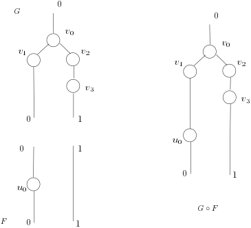
In the Figure 1, $F$ is a forest where $u_0$ is a inner node, roots are ${0, 1}$ and sites are ${0, 1}$.
The forest is made of two trees, namely two non connected subgraphs. On the right, we see the result of composing $G$ and $F$ together: $F$’s roots are glued with $G$’s sites sharing the same name.

Let us assume vertices can be enumerated, i.e. we uniquely assign a column/row index to each vertex. We carefully abuse the notation here. For example we write $M(x,y)$ for labels $x, y$ instead of using the indices associated to $x$ and $y$. We will see in a next post how to formalize that a bit better, but for now we want to explain the basic idea without too obfuscating formal notation.

An $(R,S)$-forest $F = (R \uplus S \uplus U, E)$ can be represented as a $2$-matrix $M: |S \uplus U| \to |R \uplus U|$ built in this way.

1. Assign $S$ sites to rows $\underline{|S|}$ and $U$ inner nodes to rows $|S|+\underline{|U|}$,
2. Assign $R$ roots to columns $\underline{|R|}$ and $U$ inner nodes to columns $|R|+\underline{|U|}$,
3. $M(x,y) = (y, x) \in E$, i.e. $y$ is the parent of $x$.

Basically, $M$ is the adjacency matrix of the forest. We denote $[F]$ the matrix corresponding to a forest $F$.

Graphs $F$ and $G$ in Figure 1 can be represented as two matrices $M$ and $N$, respectively.

$$
M =
\begin{array}{cc}
\begin{array}{ccc} 0 \quad 1 \quad u_0 \end{array}\
\left(\begin{array}{cc|c}
0 & 0 & 1 \
0 & 1 & 0 \
1 & 0 & 0
\end{array}\right) &
\begin{array}{c} 0 \ 1 \ u_0 \end{array}
\end{array}
$$

$$
N =
\begin{array}{cc}
\begin{array}{ccccc} 0 \quad v_0 \quad v_1 \quad v_2 \quad v_3 \end{array}\
\left(\begin{array}{ccccc}
0 & 0 & 1 & 0 & 0 \
0 & 0 & 0 & 0 & 1 \
\hline
1 & 0 & 0 & 0 & 0 \
0 & 1 & 0 & 0 & 0 \
0 & 1 & 0 & 0 & 0 \
0 & 0 & 1 & 0 & 0 \
\end{array}\right) &
\begin{array}{c} 0 \ 1 \ v_0 \ v_1 \ v_2 \ v_3 \end{array}
\end{array}
$$

Given an $(R,S)$-forest $G$ and an $(S,T)$-forest $F$, composition $G \circ F$ is defined as $[F] \cdot_{|S|} [G]$. If there are no inner nodes, composition boils down to classical matrix multiplication.

In our example $S={0, 1 }$ and $i=2$, we have separated with a line the two sub-matrices $M^{\underline{i}}$ and $N_{\underline{i}}$ induced by $S$. The partial product $M \cdot_i N$ is the following matrix.

$$
M \cdot_i N =
\begin{array}{cc}
\begin{array}{ccccc} 0 \quad v_0 \quad v_1 \quad v_2 \quad v_3 \quad u_0 \end{array}\
\left(\begin{array}{ccccc|c}
0 & 0 & 0 & 0 & 0 & 1 \
0 & 0 & 0 & 0 & 1 & 0 \
0 & 0 & 1 & 0 & 0 & 0 \
\hline
1 & 0 & 0 & 0 & 0 & 0 \
0 & 1 & 0 & 0 & 0 & 0 \
0 & 1 & 0 & 0 & 0 & 0 \
0 & 0 & 1 & 0 & 0 & 0 \
\end{array}\right) &
\begin{array}{c} 0 \ 1 \ u_0 \ v_0 \ v_1 \ v_2 \ v_3 \end{array}
\end{array}
$$

We have separated the four sub-matrices of the definition above with vertical and horizontal lines. It is easy to verify that the matrix corresponds to the composition of the two trees of this example.

In Milner, tensor product is defined if interfaces are disjoint. We define tensor product always up to renaming of interfaces (i.e. disjoint sum of names). Given an $(R,S)$-forest $G$ and an $(T, V)$-forest $F$, the tensor product $G \otimes F$ is a $(R+T, S+V)$-forest whose matrix $[G \otimes F]$ is $[F] \circ_\emptyset [G]$.

It is not hard to see that $\cdot_\emptyset$ is the matricial tensor product and it is equivalent to the juxtaposition of two trees (e.g. parallel composition).

Not every matrix is a forest, of course. In order to enforce that we need to require two additional properties on $M$:

1. $M$ is functional,
2. $M^{N}_{N}$ is acyclic.

Port graphs

Partial product applies to matrices in general. So we can model more generic data structure relaxing the acyclic condition that defines trees and forests. This leads us to the example of port graphs.

Port graphs are graphs whose vertices have ports and edges connect different ports. Formally, an $(X, Y)$-port graph $G$ is $(V, E, \mathit{ctrl}, \mathit{link})$ where $V$ is a set of vertices, $E$ a set of edges, $\mathit{ctrl}: V \to \mathbb{N}$ and $\mathit{link}: X \cup P \to Y \cup E$ where $P={ (v, i) ;|; v \in V \wedge i \in \underline{\mathit{ctrl}(v)} }$.

An $(X, Y)$-port graph $G$ can be represented as a functional matrix $L: |X \uplus P| \to |Y \uplus E|$ built in this way.

1. Assign $X$ inner names to rows $\underline{|X|}$ and $P$ ports to rows $|X|+\underline{|P|}$,
2. Assign $Y$ outer names to columns $\underline{|Y|}$ and $E$ edges to columns $|Y|+\underline{|E|}$,
3. $L(x, y) = 1$ if and only if $\mathit{link}(x) = y$.

We can compose port graphs by product as we did for forests.

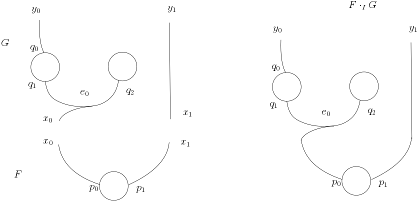
Composition of port graphs is the partial product of their respective matrices.

Partial sum

Partial product preserves acyclic and functional properties of matrices. Now we define partial sum where functionality is not preserved. Partial sum is a generalization of Milner’s parallel product. Note that Milner’s parallel product preserves functionality.

We define sum on sub-matrices. Let $M: m \to n$ and $N: k \to l$ be two matrices and $i \leq m, k$ and $j \leq n, j$, then the partial sum $+_i^j$ of $M$ and $N$ is a $m+k-i \times n+l-j$ matrix $M +_i^j N$ of this form:

$$
M +i^j N =
\begin{array}{cc}
\begin{array}{ccc} \underline{j} & \quad \underline{n} \setminus j \quad \underline{l} \setminus j \end{array}\
\left(\begin{array}{ccc}
M{\underline{i}}^{\underline{j}} + N_{\underline{i}}^{\underline{j}} & M_{\underline{i}}^{\underline{n} \setminus j} & N_{\underline{i}}^{\underline{l} \setminus j} \
M_{\underline{m}-i}^{j} & M_{\underline{n} \setminus i}^{\underline{n} \setminus j} & 0 \
N_{\underline{n} \setminus i}^{\underline{j}} & 0 & N_{\underline{k} \setminus i}^{\underline{l} \setminus j}
\end{array}\right) &
\begin{array}{c} \underline{i} \ \underline{m} \setminus i \ \underline{k} \setminus i \end{array}
\end{array}
$$

If $i = j = 0$, then $+_i^j$ is the tensor product. If $i=m=k$ and $j=n=l$, partial sum is the classical matrix sum operation.

The definition above remembers Milner’s definition of parallel product when $M_{\underline{i}}^{\underline{j}} = N_{\underline{i}}^{\underline{j}}$.

If $M: m \to n$ and $N: k \to l$ are two matrices, there are four ways (up to isomorphism?) to compose them: $M \cdot_i N$, $M \cdot_i N$, $M +_i^0 N$ ($N +_i^0 M$) and $M +_0^i N$ ($N +_0^i M$) for some proper $i$. The four ways are equivalent and correspond to tensor product when $i=0$. If we think in terms of interfaces from the examples above, the four ways are equivalent when interfaces are fully disjoint.

Final notes

Place graphs and link graphs are (surprise, surprise!) special cases of forests and port graphs, respectively.

The underlying matrix for place graphs is functional and cyclic whereas for link graphs is only functional. We can relax both conditions and define an algebra on generic matrices.

Link graph interfaces are finite set of names and not ordinals. In theory, ordinals and finite sets of names are the same (i.e. isomorphic). However, in practice, it might be convenient to have finite sets of names instead of anonymous numbers. As it is discussed in the Appendix of [1], we can define parallel composition with name sharing. From a categorical view point, this means that the wanted symmetry is achieved without cumbersome switch morphisms, which sounds lovely.

So, what if we want to replace ordinals with finite sets?

We could extend the definition of matrix with named columns and rows. For example, an $(X, Y, R)$ matrix $M$ is a function $M: X \times Y \to R$. We say $M$ ranges over finite sets $X$ and $Y$ and has values in some rig $R$. We define $\mathit{size} ; M$ as $|X| \times |Y|$.

Partial product and sum are more or less defined as above. We should pay attention to name clashing, though. So we need to define disjoint union of name sets. I do not find this approach convincing, since it makes the notation heavier. So what I will try next is the keep bare matrices as “semantic” referents and build the mapping between names and ordinals on the top of that.

References

[1] Robin Milner. The space and motion of communicating agents. Cambridge University Press, 2009.

[2] Brendan Fong and David I. Spivak. “Seven Sketches in Compositionality: An Invitation to Applied Category Theory.” arXiv preprint arXiv:1803.05316 (2018).

[3] Michele Sevegnani and Muffy Calder. “Bigraphs with sharing.” Theoretical Computer Science 577 (2015): 43-73.